Mitochondria Segmentation
Introduction
Mitochondria are the primary energy providers for cell activities, thus essential for metabolism. Quantification of the size and geometry of mitochondria is not only crucial to basic neuroscience research, but also informative to the clinical studies of several diseases including bipolar disorder and diabetes.
This tutorial has two parts. In the first part, you will learn how to make pixel-wise class prediction on the widely used benchmark dataset released by Lucchi et al. in 2012. In the second part, you will learn how to predict the instance masks of individual mitochondrion from the large-scale MitoEM dataset released by Wei et al. in 2020.
Semantic Segmentation
This section provides step-by-step guidance for mitochondria segmentation with the EM benchmark datasets released by Lucchi et al. (2012). We consider the task as a semantic segmentation task and predict the mitochondria pixels with encoder-decoder ConvNets similar to the models used in affinity prediction in neuron segmentation. The evaluation of the mitochondria segmentation results is based on the F1 score and Intersection over Union (IoU).
Note
Different from other EM connectomics datasets used in the tutorials, the dataset released by Lucchi et al. is an isotropic dataset, which means the spatial resolution along all three axes is the same. Therefore a completely 3D U-Net and data augmentation along z-x and z-y planes besides x-y planes are preferred.
All the scripts needed for this tutorial can be found at pytorch_connectomics/scripts/. Need to pass the argument --config-file configs/Lucchi-Mitochondria.yaml during training and inference to load the required configurations for this task.
The pytorch dataset class of lucchi data is connectomics.data.dataset.VolumeDataset.
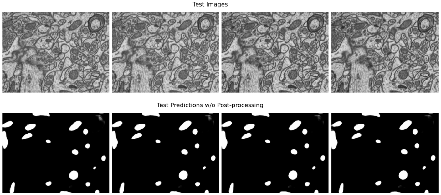
Qualitative results of the model prediction on the mitochondria segmentation dataset released by Lucchi et al., without any post-processing.
1 - Get the data
Download the dataset from our server:
wget http://rhoana.rc.fas.harvard.edu/dataset/lucchi.zip
For description of the data please check the author page.
2 - Run training
source activate py3_torch
CUDA_VISIBLE_DEVICES=0,1,2,3 python -u -m torch.distributed.run \
--nproc_per_node=4 --master_port=2345 scripts/main.py --distributed \
--config-file configs/Lucchi-Mitochondria.yaml
Similar to the neuron segmentation tutorial, we use distributed data-parallel training considering its high efficiency, and also to enable synchronized batch normalization (SyncBN).
3 - Visualize the training progress
tensorboard --logdir outputs/Lucchi_UNet/
4 - Inference on test data
source activate py3_torch
CUDA_VISIBLE_DEVICES=0,1,2,3,4,5,6,7 python -u scripts/main.py \
--config-file configs/Lucchi-Mitochondria.yaml --inference \
--checkpoint outputs/Lucchi_UNet/volume_100000.pth.tar
5 - Run evaluation
Since the ground-truth label of the test set is public, we can run the evaluation locally:
from connectomics.utils.evaluation import get_binary_jaccard
pred = pred / 255. # output is casted to uint8 with range [0,255].
gt = (gt!==0).astype(np.uint8)
thres = [0.4, 0.6, 0.8] # evaluate at multiple thresholds.
scores = get_binary_jaccard(pred, gt, thres)
The prediction can be further improved by conducting median filtering to remove noise:
from connectomics.utils.evaluate import get_binary_jaccard
from connectomics.utils.process import binarize_and_median
pred = pred / 255. # output is casted to uint8 with range [0,255].
pred = binarize_and_median(pred, size=(7,7,7), thres=0.8)
gt = (gt!==0).astype(np.uint8)
scores = get_binary_jaccard(pred, gt) # prediction is already binarized
Our pretained model achieves a foreground IoU and IoU of 0.892 and 0.943 on the test set, respectively. The results are better or on par with state-of-the-art approaches. Please check BENCHMARK.md for detailed performance comparison and the pre-trained models.
Instance Segmentation
This section provides step-by-step guidance for mitochondria segmentation with our benchmark datasets MitoEM.
We consider the task as 3D instance segmentation task and provide three different confiurations of the model output.
The model is UNet3D, similar to the one used in neuron segmentation.
The evaluation of the segmentation results is based on the AP-75 (average precision with an IoU threshold of 0.75).
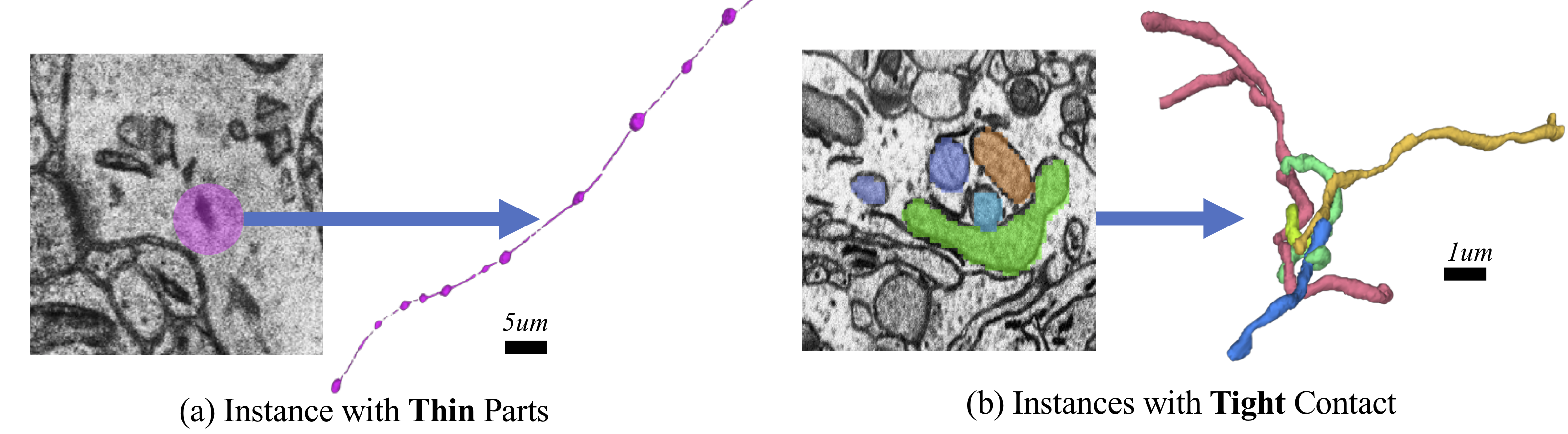
Complex mitochondria in the MitoEM dataset:(a) mitochondria-on-a-string (MOAS), and (b) dense tangle of touching instances. Those challenging cases are prevalent but not covered in previous datasets.
Note
The MitoEM dataset has two sub-datasets MitoEM-Rat and MitoEM-Human based on the source of the tissues. Three training configuration files on MitoEM-Rat
are provided in pytorch_connectomics/configs/MitoEM/ for different learning setting as described in this paper.
Tip
Since the dataset is very large and can not be directly loaded into memory, we designed the connectomics.data.dataset.TileDataset class that only
loads part of the whole volume each time by opening involved PNG or TIFF images.
1 - Dataset introduction
The dataset is publicly available at both the project page and the MitoEM Challenge page. Dataset description:
im: includes 1,000 single-channel*.pngfiles (4096x4096) of raw EM images (with a spatial resolution of 30x8x8 nm). The 1,000 images are splited into 400, 100 and 500 slices for training, validation and inference, respectively.mito_train/: includes 400 single-channel*.pngfiles (4096x4096) of instance labels for training. Similarly, themito_val/folder contains 100 slices for validation. The ground-truth annotation of the test set (rest 500 slices) is not publicly provided but can be evaluated online at the MitoEM challenge page.
To run training, JSON files containing the metadata of the dataset (for both images and labels) need to be provided. Example
JSON files can be found in configs/MitoEM.
2 - Model configuration
Configure *.yaml files for different learning targets:
MitoEM-R-A.yaml: output 3 channels for predicting the affinty between voxels.MitoEM-R-AC.yaml: output 4 channels for predicting both affinity and instance contour.MitoEM-R-BC.yaml: output 2 channels for predicting both the binary foreground mask and instance contour. This configuration achieves the best overall performance according to our experiments.
3 - Run training
We show examples for running the training script for the U3D-BC model:
Note
By default the path of images and labels are not specified. To
run the training scripts, please revise the DATASET.IMAGE_NAME, DATASET.LABEL_NAME, DATASET.OUTPUT_PATH
and DATASET.INPUT_PATH options in configs/MitoEM/MitoEM-R-*.yaml.
The options can also be given as command-line arguments without changing of the yaml configuration files.
CUDA_VISIBLE_DEVICES=0,1,2,3 python -u -m torch.distributed.run \
--nproc_per_node=4 --master_port=4321 scripts/main.py --distributed \
--config-base configs/MitoEM/MitoEM-R-Base.yaml \
--config-file configs/MitoEM/MitoEM-R-BC.yaml
4 - Visualize the training progress
We use TensorBoard to visualize the training progress. For Harvard FASRC cluter users, more info can be found here.
tensorboard --logdir outputs/MitoEM_R_BC/
5 - Run inference
Run inference on validation/test image volumes (suppose the model is optimized for 100k iterations):
python -u scripts/main.py \
--config-base configs/MitoEM/MitoEM-R-Base.yaml \
--config-file configs/MitoEM/MitoEM-R-BC.yaml --inference \
--checkpoint outputs/MitoEM_R_BC/checkpoint_100000.pth.tar
Note
Please change the INFERENCE.IMAGE_NAME INFERENCE.OUTPUT_PATH INFERENCE.OUTPUT_NAME
options in configs/MitoEM-R-*.yaml based on your own data path.
6 - Post-process
The post-processing step requires merging output volumes and applying watershed segmentation.
As mentioned before, the dataset is very large and can hardly be directly loaded into memory for
processing. Therefore our code run prediction on smaller chunks sequentially, which produces
multiple *.h5 files with the coordinate information. To merge the chunks into a single volume
and apply the segmentation algorithm:
import glob
import numpy as np
from connectomics.data.utils import readvol
from connectomics.utils.process import bc_watershed

output_files = 'outputs/MitoEM_R_BC/test/*.h5' # output folder with chunks
chunks = glob.glob(output_files)

vol_shape = (2, 500, 4096, 4096) # MitoEM test set
# vol_shape = (2, 100, 4096, 4096) # MitoEM validation set
pred = np.ones(vol_shape, dtype=np.uint8)
for x in chunks:
    pos = x.strip().split("/")[-1]
    print("process chunk: ", pos)
    pos = pos.split("_")[1].split("-")
    pos = list(map(int, pos))
    chunk = readvol(x)
    pred[:, pos[0]:pos[1], pos[2]:pos[3], pos[4]:pos[5]] = chunk

# This function process the array in numpy.float64 format.
# Please allocate enough memory for processing.
segm = bc_watershed(pred, thres1=0.85, thres2=0.6, thres3=0.8, thres_small=1024)
Note
The decoding parameters for the watershed step are a set of reasonable thresholds but not optimal given different segmentation models. We suggest conducting a hyper-parameter search on the validation set to decide the decoding parameters.
Then the segmentation map should be ready to be submitted to the MitoEM challenge website for evaluation. Please note that this tutorial only take the MitoEM-Rat set as an example. The MitoEM-Human set also need to be segmented for online evaluation.
7 - Evaluate on the validation set
The performance of the MitoEM test sets can only be evaluated on the challenge website. Dataset users are encouraged to experiment
with the metric code on the validation set to understand the evaluation function and conduct a hyper-parameter search.
Evaluation is performed with the demo.py file provided by the mAP_3Dvolume repository.
The ground truth .h5 file can be generated from the 2D images using the following script:
import glob
import numpy as np
from connectomics.data.utils import writeh5, readvol

gt_path = "datasets/MitoEM_R/mito_val/*.tif"
files = sorted(glob.glob(gt_path))

data = []
for i, file in enumerate(files):
    print("process chunk: ", i)
    data.append(readvol(file))

data = np.array(data)
writeh5("validation_gt.h5", data)
The resulting scores can then be obtained by executing python demo.py -gt /path/to/validation_gt.h5 -p /path/to/segmentation_result.h5
